Reproducible data ingestion in practice
How does a reproducible data ingestion look like in practice?
If your analytical work has used a certain type of data at least two times in the past, it is likely that the data will be needed again. This is a good time to make the data ingestion automatic and reproducible. We demonstrate a simple data ingestion from Eurostat. I am a contributor and developer of the rOpenGov collective that maintains the eurostat package for reproducible access to the European statistical agencies data warehouse, and my other packages iotables for national accounts data in input-output analysis and regions for regional statistics.
library(eurostat)
nuts3_population_raw <- get_eurostat ("demo_r_pjangrp3")
nuts3_population_metadata <- get_eurostat_toc() %>%
  filter ( code == "demo_r_pjangrp3" ) %>%
  distinct_all ()

last_update <- nuts3_population_metadata$`last update of data`
first_data <- nuts3_population_metadata$`data start`
The metadata entries to this statistics suggest that the latest data is from Thursday 14 May, 2020, so it is high time to refresh your data tables and update your charts. Sadly, the metadata suggest that on this occasion the table went through structural changes, so you may get a different spreadsheet table when you downloaded compared to the last occasion. You may think that this is another reason to automate the ingestion into a well-defined, tidy table format.
| title | code | last update of data | last table structure change | data start | data end |
|---|---|---|---|---|---|
| Population on 1 January by age group, sex and NUTS 3 region | demo_r_pjangrp3 | 14.05.2020 | 14.05.2020 | 2014 | 2019 |
Looking at the head of this raw data, you realize that this is not table, but a little database! It contains population divisions by sex and age groups. However, your indicator is the total population of each NUTS3 regions, so let’s filter out only the total population for both sexes.
| sex | unit | age | geo | time | values |
|---|---|---|---|---|---|
| T | NR | Y_LT5 | NO07 | 2018-01-01 | 25108 |
| M | NR | Y10-14 | DED44 | 2014-01-01 | 4620 |
| F | NR | Y45-49 | FRB | 2014-01-01 | 88590 |
Looking at the head of this raw data, you realize that this is not table, but a little database! It contains population divisions by sex and age groups. However, your indicator is the total population of each NUTS3 regions, so let’s filter out only the total population for both sexes.
nuts3_population <- nuts3_population_raw %>%
  filter ( sex == "T",             # for both sexes
           age == "TOTAL") %>%     # for all age groups
  mutate ( year = as.integer(substr(as.character(time), 1,4)),
           indicator = paste0("population_sex-", sex, "_unit-", unit,
                               "_age-", age)) %>%
  select ( -all_of(c("sex", "unit", "age")))
The following table is already tidy — each observation corresponds with a small region of Europe. The filtering information as metadata is included in the indicator’s name.
| geo | time | values | year | indicator |
|---|---|---|---|---|
| HU222 | 2015-01-01 | 253997 | 2015 | population_sex-T_unit-NR_age-TOTAL |
| NO | 2014-01-01 | 5107970 | 2014 | population_sex-T_unit-NR_age-TOTAL |
| ES704 | 2016-01-01 | 112087 | 2016 | population_sex-T_unit-NR_age-TOTAL |
| FRK12 | 2015-01-01 | 146219 | 2015 | population_sex-T_unit-NR_age-TOTAL |
| DE3 | 2018-01-01 | 3613495 | 2018 | population_sex-T_unit-NR_age-TOTAL |
| NL225 | 2019-01-01 | 400685 | 2019 | population_sex-T_unit-NR_age-TOTAL |

The population size is rather homogeneous — no wonder, the small regions of Europe are exactly defined to be roughly of equal size and easily comparable.
You are wondering how you could match this data with your own records, or data acquired from Google about number of restaurants or searchers for concerts?
| geo | time | values | year | indicator |
|---|---|---|---|---|
| IE042 | 2017-01-01 | 451293 | 2017 | population_sex-T_unit-NR_age-TOTAL |
| SI044 | 2014-01-01 | 112848 | 2014 | population_sex-T_unit-NR_age-TOTAL |
| DE225 | 2015-01-01 | 77927 | 2015 | population_sex-T_unit-NR_age-TOTAL |
| PL621 | 2016-01-01 | 523096 | 2016 | population_sex-T_unit-NR_age-TOTAL |
| TRB13 | 2018-01-01 | 273354 | 2018 | population_sex-T_unit-NR_age-TOTAL |
| FRK24 | 2018-01-01 | 1261373 | 2018 | population_sex-T_unit-NR_age-TOTAL |
There is no easy solution for this problem. Within the EU in the last 20 years there were several thousand internal boundary changes — states, provinces, regions are rather free to change their internal administration boundaries. Regions are constantly changing their names or their spelling, too. Sometimes they use a standard English translation of their region, sometimes only the national language variants. In Greece or Bulgaria they do not even use the Latin alphabet!
With Istvan we have created and released an open-source code library, regions to deal with similar issues. It allows the changes between boundary definition between 1999-2021, or the connection of the globally used geographical typology adopted by Google with Eurostat’s EU-only definitions.
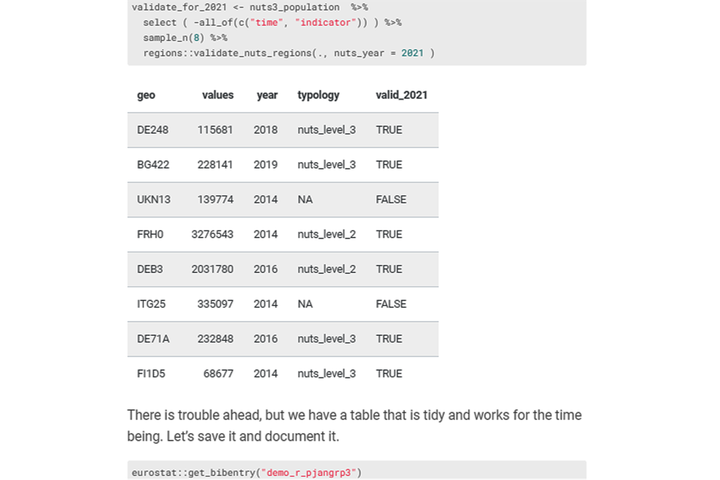
For example, you can already foresee that there are future changes (to be implemented from the year 2021) that will affect two of these regions.
set.seed(21)
validate_for_2021 <- nuts3_population  %>%
  select ( -all_of(c("time", "indicator")) ) %>%
  sample_n(8) %>%
  regions::validate_nuts_regions(., nuts_year = 2021 )
| geo | values | year | typology | valid_2021 |
|---|---|---|---|---|
| DE248 | 115681 | 2018 | nuts_level_3 | TRUE |
| BG422 | 228141 | 2019 | nuts_level_3 | TRUE |
| UKN13 | 139774 | 2014 | NA | FALSE |
| FRH0 | 3276543 | 2014 | nuts_level_2 | TRUE |
| DEB3 | 2031780 | 2016 | nuts_level_2 | TRUE |
| ITG25 | 335097 | 2014 | NA | FALSE |
| DE71A | 232848 | 2016 | nuts_level_3 | TRUE |
| FI1D5 | 68677 | 2014 | nuts_level_3 | TRUE |
There is trouble ahead, but we have a table that is tidy and works for the time being. Let’s save it and document it.
eurostat::get_bibentry("demo_r_pjangrp3")
## @Misc{demo_r_pjangrp3_14-05-2020,
##   title = {Population on 1 January by age group, sex and NUTS 3 region [demo_r_pjangrp3]},
##   url = {https://ec.europa.eu/eurostat/web/products-datasets/-/demo_r_pjangrp3},
##   language = {en},
##   year = {14.05.2020},
##   publisher = {Eurostat},
##   author = {{Eurostat}},
##   urldate = {2020-07-25},
## }
What is reproducibility in this case?
Replicability means that somebody else in your team can get exactly the same data as in this post.
- Recording exactly what have your analysts downloaded, including source, date, filtering settings
Reproducibility means that not only your team, but an external auditor or a peer reviewer can easily validate that your data is sound. All our solutions are opens source, and use the most popular statistical programming language, R. Anybody with a basic knowledge of R, or probably even SQL (we use an extension of R that uses SQL-like syntax) can read if everything goes allright. Your team can even modify the code.
- Creating a documentation that you updates your reports data citations
Confirmability means that somebody who is not using . All our solutions are opens source, and use the most popular statistical programming language, R. R is supported by Microsofts BI products, SPSS and other statistical software, too. We are not a software company, there is no vendor lock-in, and our work can be confirmed with other statistical software.
- Data acquired via our data gathering apps is automatically documented, follows tidy formats and valid abbreviations, and can be confirmed in a wide range of statistical and spreadsheet applications, including SPSS, Excel, OpenOffice, Google Spreadsheets.
- Bringing the data to a tidy format which is easy to join with other data in a spreadsheet application, or stored in a relational database.
- Validating the data structure, in this case, with special attention to regional boundaries and regional names.
Auditability means that external auditors can validate that the data your team uses from our app is correct.
- We are following methodological guidelines and definitions set by international bodies such as Eurostat’s ESSNet statistical network or IFRS.
- Our critical software code is not only open source, but goes through various levels of statistical peer-review. We are sending for scientific validation and peer-review our methodology, too.
- Being open source allows us to make any corrections, updates, should any problem or standard change affect the data.
References
Antal, Daniel. 2020. Regions: Processing Regional Statistics. https://regions.danielantal.eu/.
Eurostat. n.d. Eurostat. Accessed July 25, 2020. https://ec.europa.eu/eurostat/web/products-datasets/-/demo_r_pjangrp3.
Lahti, Leo, Janne Huovari, Markus Kainu, and Przemyslaw Biecek. 2020. Eurostat: Tools for Eurostat Open Data. https://CRAN.R-project.org/package=eurostat.
Hadley Wickham. 2014. Tidy Data.Journal of Statistical Software vol 59, no 10.https://www.jstatsoft.org/v059/i10.